Who are Trump’s people?  While bricks may be the building blocks to Trump’s skyscrapers, we’re going to use statistics to see what demographics are the building blocks of someone who likes Donald Trump. 

In 0ptimus’ survey last week among likely Republican voters in New York and Wisconsin, I asked them about their feelings toward Donald Trump.

“Thinking about Donald Trump, which of the following best describes your opinion of him?”

The answer choices, randomized to avoid bias, were “strongly favorable,” “somewhat favorable,” “no opinion,” “somewhat unfavorable,” and “strongly unfavorable.”  Note that this isn’t about ballot test support (i.e. If the election were held tomorrow, who would you vote for?) but about favorability.  Favorability often precedes ballot test support.  For example, if you supported Ben Carson, you would likely need to find a new candidate to support in the election once Carson dropped out.  If you had a very favorable opinion toward Trump and Rubio but a very unfavorable opinion toward Cruz, it is very unlikely that you would become a Cruz supporter and likelier that you would support either Trump or Rubio.

After asking the above favorability question, I wanted to find out what makes someone favorable toward Trump.  I used a technique called “ordinal logistic regression” to build a model and quantify how strongly different variables could predict being favorable toward Trump.  Ordinal logistic regression, in broad strokes, is a type of model designed to predict a categorical variable that has some type of order or ranking attached to it.  In this case, our categorical variable is Trump favorability, the five categories are strongly favorable/somewhat favorable/no opinion/somewhat unfavorable/strongly unfavorable and these are ordered from most favorable to least favorable.  (An example of a non-ordered categorical variable would be classifying people by what they believe the top threat to national security is: China, Russia, or ISIS.  There isn’t some ordering where one group is “greater than” or “less than” the others.)

Based on available income, sex, age, ethnicity, voting history, and Congressional district data, I constructed a model for both New York and Wisconsin.  Since the ordinal logistic regression model is more complicated than those generally published, interpretation isn’t as straightforward as models you may have seen before.  I want to focus on interpretability and will paint in broad strokes below but will provide the information available for those interested in diving into the nitty-gritty details of odds ratios and statistical inference.

Our goal is to see how changing one variable (i.e. age, Congressional district, income) affects one’s favorability toward Trump.  The odds ratio is a measure of association between two variables by comparing two groups: our “group of interest” and our “reference group.”  For a quantitative variable like age, the group of interest will be people who are 1 year older with everything else held equal and the reference group will be people who are 1 year younger with everything else equal.  For a categorical variable like ethnicity, the reference group is the one left out of the table (in Tables 1 and 2, White) and the group of interest will differ depending on which row of the table to which you’re looking.  We’ve included a column of “reference groups” in Tables 1 and 2.  Referencing Table 1 and 2, the “OR Estimate” column is our data-based estimate of the true odds ratio.  Broadly speaking, if the OR estimate is around 1, there isn’t a difference between the group of interest and the reference group.  The “p-value” column measures how confident we are that the true odds ratio (not our estimate in the table) is significantly different from 1.  A low p-value (lower than 1%, 5%, or 10%) means we’re very sure that the true odds ratio will be different from 1.  A p-value that is higher than 10% means that our OR estimate is too close to 1 to conclude the true odds ratio is different from 1 and it suggests we shouldn’t put much stock into that particular odds ratio estimate.  If the OR estimate is larger than 1 and the p-value is low, then the group of interest is, on average, more likely to be more favorable toward Trump.  If the OR estimate is smaller than 1 and the p-value is low, then the group of interest is, on average, less likely to be more favorable toward Trump. We’ve provided the “LOR Estimate” (log-odds ratio estimate), “Std. Error” (standard error on LOR scale), “t score” and information for the intercepts for the statistically savvy, but glossing over these doesn’t affect understanding the ideas here.

Now that we have some numbers to work with, we can look at what groups of people tend to like Trump.

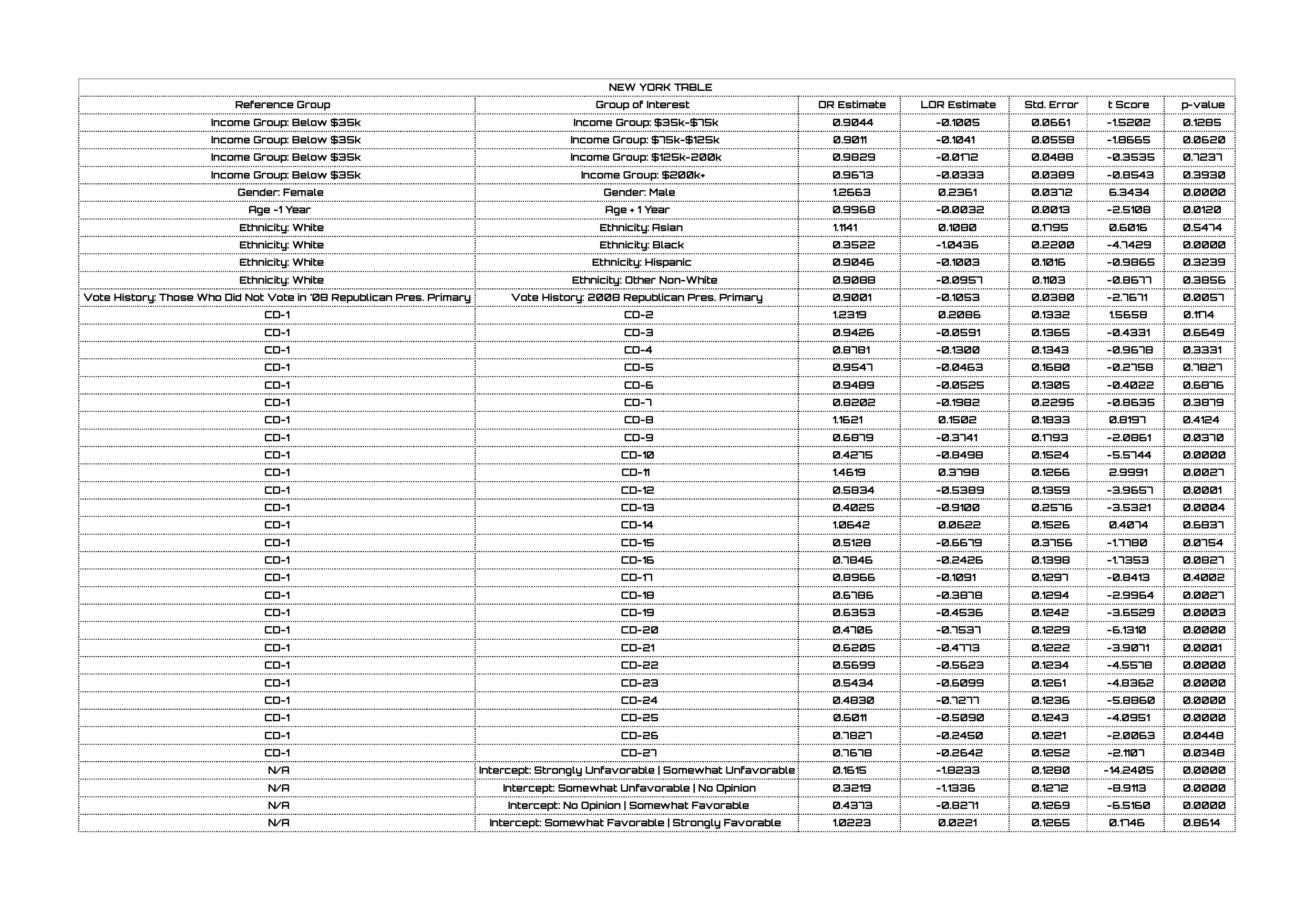
Table 1 – Results of Ordinal Logistic Regression Model in New York (click to enlarge)

First and foremost, income group appears to be a poor predictor of who likes Donald Trump.  Given Trump’s personal wealth (and his flagrant displays of it), one might think that his message may resonate differently with voters of different economic backgrounds.  This data suggests that isn’t the case; among New York voters, the only group that is significantly different than those making less than $35,000 a year is the group making between $75,000 and $125,000 a year – and even though there’s a “statistically significant” difference here, the “real-world” difference is pretty small.

Much more notable is the difference between men and women.  The odds ratio for men relative to women is 1.27, which means men are 1.27 times as likely to like Trump as women – an important issue when you consider that women make up 49.4% of our likely voter universe and, as estimated from our voter file, 54.8% of all registered voters in New York.  (My colleague Haley went much more in depth on the Donald Trump vs. women issue; you should check her post out.)

As people get older, they become less likely to be favorable toward Trump.  The odds ratio looks very close to 1, but a) the p-value is very small and b) we need to remember that this only looks at the difference of one year.  Looking at the difference between five years, ten years, or a generation will tell a very different story.

The only ethnicity that is significantly different from White voters (with respect to Trump’s favorability) is Black – and it looks as though Black people are wayy (yeah, two Ys warranted) less likely to like Trump.  White voters are three times as likely to like Trump as Black voters.  I’m not shocked by this difference considering the, um, things Trump says.  What I am shocked by is the lack of a difference between White voters and Hispanic voters, based on the p-value.

Vote history seems to be a significant predictor of Trump favorability; those who voted in the 2008 Republican presidential primary are 90% as likely to like Trump as those who did not vote in 2008.

We can also see that there are major differences in Trump favorability among the different Congressional districts in New York.

 

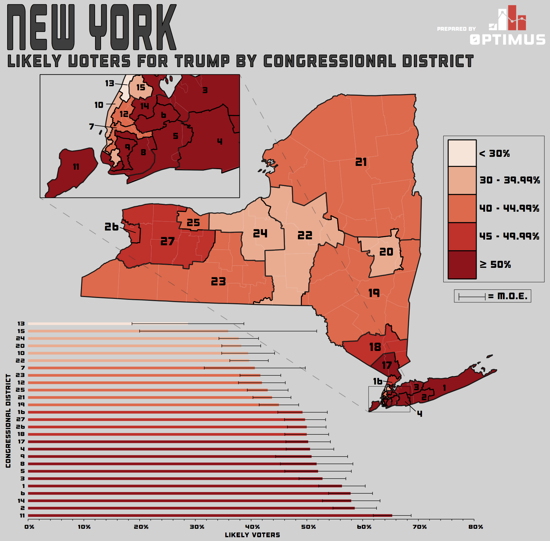
Figure 1 – Map of Trump Favorability Across New York Congressional Districts (click to enlarge)

Fifteen of the 27 Congressional districts are significantly different from New York’s 1st Congressional District when it comes to Trump favorability.  Given the different shades of red indicating the different levels of Trump ballot test support across the state of New York in Figure 1, we shouldn’t be surprised that favorability levels are very different as well.  (To reiterate, ballot test support and favorability are not the same thing – but they are obviously highly associated with one another.)

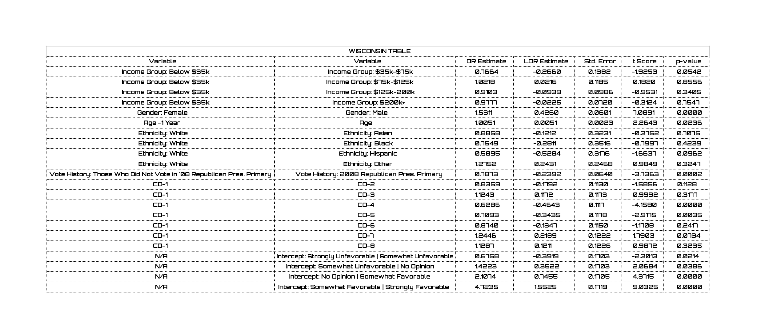
Table 2 – Results of Ordinal Logistic Regression Model in Wisconsin (click to enlarge)

Shifting to Wisconsin, we see a very similar story.  Only one income group is statistically different from those making below $35,000 a year; interestingly it is the next-most-profitable group – those making between $35,000 and $75,000 a year.  The difference between men and women is even more pronounced in Wisconsin; men are 1.53 times as likely as women to be favorable toward Trump.  Similarly, those who voted in 2008’s Presidential primary are worse for Trump in Wisconsin than New York – those who did vote in 2008 are 78% as likely to support him as those who did not vote (compared to New York’s 90%).

In Wisconsin, we see what I expected to see in New York: Hispanic voters are much 59% as likely to like Trump as White voters.  We also see the same geographic disparity we saw in New York in that different Congressional districts – made up of different populations with different demographic make-ups – vary wildly in their favorability toward Trump.

 

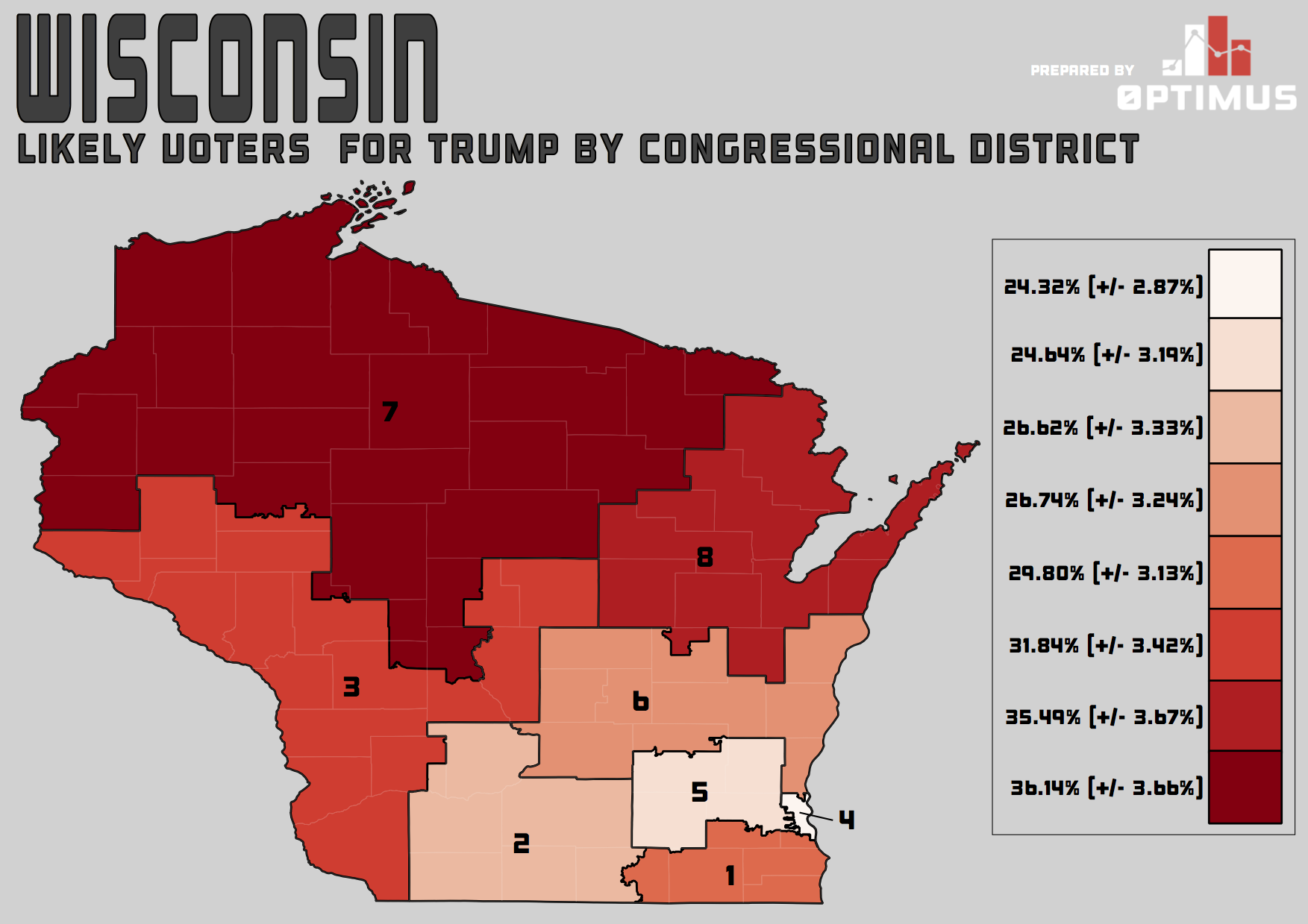
Figure 2 – Map of Trump Favorability Across Wisconsin Congressional Districts (click to enlarge)

All of these above statements – in both New York and Wisconsin – assume that everything else is held equal.  For example, the odds ratio for men to women in New York (1.27) assumes that if we were considering two people, their sex differs but their age, ethnicity, income, etc. all stay exactly the same.  Rarely is this actually the case; while it will go beyond this blog post-turned-novel to actually assess how significant the difference is, those who fall into multiple “less likely to like Trump” categories are probably going to be more anti-Trump than those who fall into only one of the “less likely to like Trump” categories.  The same goes for those who fall into multiple “more likely to like Trump” categories.

As far as elections go, while I don’t advise rewriting strategies based on “identity politics,” I think it would behoove Trump to check the direction of the wind by licking his finger or seeing which way his hair is pointing and realize that what he’s saying might possibly have some negative effect on how he’s doing with certain groups of people, especially if he fancies himself as the person who can unite the GOP.

The data sets for this analysis were the 0ptimus in-house voter files and the survey data gathered in New York and Wisconsin by IVR calls from 3.22 to 3.24.  The main method used here, ordinal logistic regression, was implemented by fitting the models in R.  Though the two-tailed p-values were calculated directly in R, a Student’s one-sample t-test was implicitly used to assess the significance of each individual predictor.